2024-heraklion-data/notebooks/020_numpy/if_time_002_broadcasting.ipynb at b8f20bf7d4272e3693f4f79a02a915d39eb05041

In [2]:

import numpy as np

def print_info(a):
    """ Print the content of an array, and its metadata. """
    
    txt = f"""
dtype\t{a.dtype}
ndim\t{a.ndim}
shape\t{a.shape}
strides\t{a.strides}
    """

    print(a)
    print(txt)

In [3]:

a = np.array([1, 2, 3])
b = np.array([[1, 2, 3], [1, 2, 3]])
a + b

Out[3]:

array([[2, 4, 6],
       [2, 4, 6]])

Broadcasting¶

The term broadcasting describes how NumPy treats arrays with different shapes during arithmetic operations

Array operations¶

NumPy operations are usually done on pairs of arrays on an element-by-element basis. Arrays of the same size are added element by element

In [4]:

x = np.array([0, 2, 4, 6])
y = np.array([1, 3, 5, 7])
print(x)
print(y)

[0 2 4 6]
[1 3 5 7]

In [5]:

x + y

Out[5]:

array([ 1,  5,  9, 13])

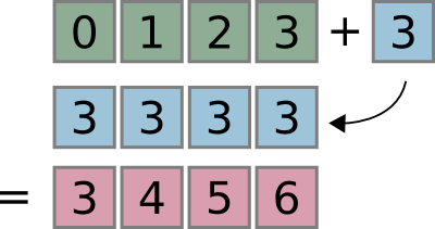
in numpy, we can just as easily add a scalar to x

In [6]:

print(x)

[0 2 4 6]

In [8]:

x + 3 # why added to the full array and not just to the first element? --> broadcasting

Out[8]:

array([3, 5, 7, 9])

In [9]:

# Alterenative 
# that no one does, hopefully
# Make a new copy of array
# Loop through array and add 3
newx = x.copy()
for i in np.arange(x.size):
    newx[i] = newx[i] + 3
print('Inefficient', newx)

print()

# Stretch out 3 to the same shape of array
# Add x + 3
new3 = [3, 3, 3, 3]
x = x + new3
print('Inefficient', x)

Inefficient [3 5 7 9]

Inefficient [3 5 7 9]

Broadcasting¶

We can think of broadcasting as an operation that stretches or duplicates the value 3 into the array [3, 3, 3, 3], and adds the results.

The code in the first example is more efficient than that in the first because broadcasting moves less memory around during the addition (3 is a scalar rather than an array)

2D broadcasting¶

In [10]:

a = np.array([1, 2, 3]) 
b = np.array([[4, 5, 6], [7, 8, 9]])

print(a)
print('')
print(b)

[1 2 3]

[[4 5 6]
 [7 8 9]]

Adding 'a' to each row of 'b'

In [11]:

a + b

Out[11]:

array([[ 5,  7,  9],
       [ 8, 10, 12]])

In [ ]:

# I don't need to loop through each row of b and add a
print('Inefficient')
for i in b:
    print(i + a)

print()

print('Inefficient')
#Or repeat a to match the dimensions of b
newa = np.array([[1, 2, 3], [1, 2, 3]])
newa = np.tile(a, (2, 1))
print(newa+b)

The advantage of NumPy's broadcasting is that this duplication of values does not actually take place, but it is a useful mental model as we think about broadcasting.

Why does understanding broadcasting matter?¶

Efficient element-wise operations with numpy
Simplifies code
Flexibly manipulate data
Understand broadcasting errors

Three rules of Broadcasting

When operating on two arrays, NumPy compares their shapes.

Rule 1: If the two arrays differ in their number of dimensions, the shape of the one with fewer dimensions is padded with ones on its leading LEFT side : Pad

Rule 2: If the shape of the two arrays does not match in any dimension, the array with shape equal to 1 in that dimension is stretched to match the other shape : Stretch

Rule 3: If in any dimension the sizes disagree and neither is equal to 1, an error is raised : Check

Pad, Stretch, Check

Broadcasting example 1¶

In [ ]:

a = np.array([1, 2, 3])
b = np.array([[4, 5, 6], [7, 8, 9]])

print(a)
print('')
print(b)

In [ ]:

print(a.shape)
print()
print(b.shape)

Rule 1: Pad¶

If the two arrays differ in their number of dimensions, the shape of the one with fewer dimensions is padded with ones on its leading (left) side

We see by rule 1 that the array a has fewer dimensions, so we pad it on the left with ones:

a.shape -> (1, 3)

b.shape -> (2, 3)

Rule 2: Stretch¶

If the shape of the two arrays does not match in any dimension, the array with shape equal to 1 in that dimension is stretched or "broadcast" to match the other shape.

By rule 2, we now see that the first dimension disagrees, so we stretch this dimension in a to match:

a.shape -> (2, 3)

b.shape -> (2, 3)

The shapes match, and we see that the final shape will be (2, 3)

Rule 3: Check¶

If in any dimension the sizes disagree and neither is equal to 1, an error is raised : Check

In [ ]:

(a+b).shape

Broadcasting example 2¶

In [ ]:

a = np.arange(3)
b = np.arange(4).reshape(4, 1)

In [ ]:

print(a.shape)
print()
print(b.shape)

In [ ]:

(a+b).shape

Broadcasting example 3¶

In [12]:

a = np.ones((3, 2))
b = np.array([4, 5, 6])

In [13]:

print(a.shape)
print()
print(b.shape)

(3, 2)

(3,)

In [14]:

(a+b).shape

---------------------------------------------------------------------------
ValueError                                Traceback (most recent call last)
Cell In[14], line 1
----> 1 (a+b).shape

ValueError: operands could not be broadcast together with shapes (3,2) (3,)

Rule 3 : Check¶

If in any dimension the sizes disagree and neither is equal to 1, an error is raised.

But numpy should have just padded on the right....

thats not how the broadcasting rules work! It would lead to potential areas of ambiguity. If right-side padding is what you'd like, you can do this explicitly by reshaping the array

In [15]:

a = np.ones((3, 2))
b = np.array([4, 5, 6])[:, np.newaxis]
# b = np.array([4, 5, 6]).reshape((3, 1))

In [16]:

print(a.shape)
print()
print(b.shape)

(3, 2)

(3, 1)

In [17]:

(a+b).shape

Out[17]:

(3, 2)

Recap¶

Scalar    2D           3D           Bad

( ,)     (3, 4)     (3, 5, 1)    (3, 5, 2)
(3,)     (3, 1)     (      8)    (      8)
----     ------     ---------    ---------
(3,)     (3, 4)     (3, 5, 8)       XXX

Mind-on exercises

Exercise 1: warm up¶

What is the expected output shape for each operation?

In [19]:

a = np.arange(5)
b = 5

np.shape(a-b)

Out[19]:

(5,)

In [21]:

a = np.ones((7, 1))
b = np.arange(7)
np.shape(a*b)

Out[21]:

(7, 7)

In [23]:

a = np.random.randint(0, 50, (2, 3, 3))
b = np.random.randint(0, 10, (3, 1))

np.shape(a-b)

Out[23]:

(2, 3, 3)

In [25]:

a = np.arange(100).reshape(10, 10)
b = np.arange(1, 10)

np.shape(a+b)

---------------------------------------------------------------------------
ValueError                                Traceback (most recent call last)
Cell In[25], line 4
      1 a = np.arange(100).reshape(10, 10)
      2 b = np.arange(1, 10)
----> 4 np.shape(a+b)

ValueError: operands could not be broadcast together with shapes (10,10) (9,)

Exercise 2¶

1. Create a random 2D array of dimension (5, 3)
2. Calculate the maximum value of each row
3. Divide each row by its maximum

Remember to use broadcasting : NO FOR LOOPS!

In [ ]:

## Your code here

Exercise 3¶

Task: Find the closest cluster to the observation.

Again, use broadcasting: DO NOT iterate cluster by cluster

In [ ]:

observation = np.array([30.0, 99.0]) #Observation

#Clusters
clusters = np.array([[102.0, 203.0],
             [132.0, 193.0],
            [45.0, 155.0], 
            [57.0, 173.0]])

Lets plot this data

In the plot below, + is the observation and dots are the cluster coordinates

In [ ]:

import matplotlib.pyplot as plt 

plt.scatter(clusters[:, 0], clusters[:, 1]) #Scatter plot of clusters
for n, x in enumerate(clusters):
    print('cluster %d' %n)
    plt.annotate('cluster%d' %n, (x[0], x[1])) #Label each cluster
plt.plot(observation[0], observation[1], '+'); #Plot observation

Closest cluster as seen by the plot is 2. Your task is to write a function to calculate this

hint: Find the distance between the observation and each row in the cluster. The cluster to which the observation belongs to is the row with the minimum distance.

distance = $\sqrt {\left( {x_1 - x_2 } \right)^2 + \left( {y_1 - y_2 } \right)^2 }$

In [ ]:

## Your code here

Sources + Resources¶

ASPP 2016 - Stéfan van der Walt - https://github.com/ASPP/2016_numpy

Basic Numpy: http://scipy-lectures.org/intro/numpy/index.html

Advanced Numpy: http://scipy-lectures.org/advanced/advanced_numpy/index.html

Numpy chapter in "Python Data Science Handbook" https://jakevdp.github.io/PythonDataScienceHandbook/02.00-introduction-to-numpy.html

28 KiB Raw Blame History

Broadcasting¶

Array operations¶

Broadcasting¶

2D broadcasting¶

Why does understanding broadcasting matter?¶

Broadcasting example 1¶

Rule 1: Pad¶

Rule 2: Stretch¶

Rule 3: Check¶

Broadcasting example 2¶

Broadcasting example 3¶

Rule 3 : Check¶

Recap¶

Exercise 1: warm up¶

Exercise 2¶

Exercise 3¶

Sources + Resources¶

28 KiB

Raw Blame History